Hierarchical Models: A Binomial Model with Shrinkage

The material in this post comes from various sources, some of which can be found in

[1] Kruschke, J. K. (2014). Doing Bayesian data analysis: A tutorial with R, JAGS, and Stan, second edition. Doing Bayesian Data Analysis: A Tutorial with R, JAGS, and Stan, Second Edition. http://doi.org/10.1016/B978-0-12-405888-0.09999-2

[2] Gelman, A., Carlin, J. B., Stern, H. S., & Rubin, D. B. (2013). Bayesian Data Analysis, Third Edition (Texts in Statistical Science). Book.

[3] Jaynes, E. T. (2003). Probability theory the logic of science. Cambridge University Press (2003)

[4] Albert, J., Gentleman, R., Parmigiani, G., & Hornik, K. (2009). Bayesian computation with R. http://doi.org/10.1007/978-0-387-92298-0

The source code for R and Stan scripts can be found at github.

In some data modelling problems with many related parameters, the dependence between these parameters can be reflected in the model. For example, if data has been collected from hospitals A, B and C; and these hospitals can be considered comparable – then we can have a structure in the model where this data can be modelled at population level, representing parameters for an entity ‘hospital’ and second level for each individual hospital A, B and C. The two concepts of exchangeability and shrinkage are briefly mentioned before talking about hierarchical models.

Exchangeability:

Consider a probability distribution  , where any index of x is the result of that trial, e.g. Red or White ball. If the probability of an event, e.g. Red on the 3rd draw is the same under any ordering of the sequence – then such a distribution is called exchangeable [3]. Chapter on elementary sampling theory in Ref [3] explains this in more detail. Such data is commonly modelled, as exchangeable, independently and identically distributed (iid), given some parameter vector Θ. This exchangeability can be extended to multiple levels in hierarchical models [2].

Shrinkage:

In structured, hierarchical models, the low level parameters (e.g. Thetas in Figure 1 below) are being affected/restrained by the higher level parameters and their subset of the data. While the higher level parameters, in turn, are affected from the data from other groups. This may lead to a reduction of variance and pulling of the low level parameters towards the common, shared high level parameters – and is called Shrinkage. It tends to affect those low level parameters more, where the data is sparse and in some cases may increase the variance, if the higher level parameters have multiple modes [1].

Rat Tumour Example:

The first example of a hierarchical model is from Chapter 5 [2]. Suppose we have rat tumour rates from 71 historic and one latest experiment, and the task is to estimate 72 probabilities of tumour, Θ, in the these rats. However the data comes from experiments performed in the same laboratory on the same strain of rats. We can model this data perhaps in 3 different ways:

• Complete Pooling: This puts all the data together and implicitly assumes that higher level distribution has a variance of zero.
• No Pooling: Each experiment is analysed separately, implicitly assuming that the higher level distribution has infinite variance.
• Partial Pooling OR Hierarchical Model: All the individual Θs can be assumed as an exchangeable sample from a common population distribution – and the unobserved population parameters can be estimated.

In a hierarchical model, there are multiple parameters being estimated at different levels, and these parameters exist in a joint parameter space. We can however factorise these joint parameter models into a chain of dependencies:

Reading from right to left, Φ is the vector of hyper-parameters (population parameters) and this is related to the parameter vector Θ, that in turn is related to the data. The figure below shows the general structure of the model.

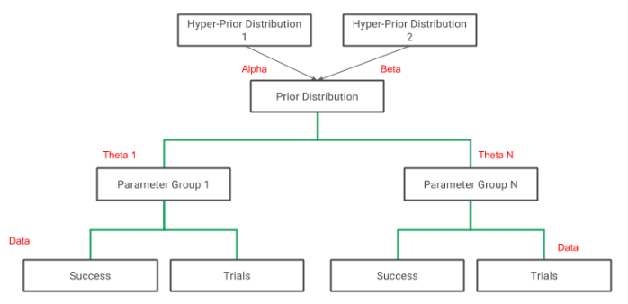
Figure 1: Structure of a 1 Level Model, from bottom to top: 1) Likelihood level, where each set of data values has a set of parameters ; 2) Each Parameter Theta is distributed as  ; 3) Hyperparameters Alpha and Beta are either fixed or have hyper-prior distributions.

This model has 1 level, one is a likelihood level (which can be called level 0) and estimates the probabilities for each experimental batch based on the data in that batch, while the higher level (population level or prior) is level 1. The main parameters of interest in this experiment are the individual theta values for each experiment (probabilities of tumour) – while in some cases the population level parameter may also be of interest, i.e. Alpha and Beta. We model the data, following the example from [2], as binomial data at the likelihood level, and the prior distribution is conjugate beta distribution (beta-binomial model). In this hierarchical model, the estimated thetas will be constrained by the structure of the model, and we are less likely to overfit the model to the data.

Estimating the Alpha and Beta parameters for the population distribution can be done in various ways, depending on the balance between complexity, computation speed and accuracy of the estimates.

Empirical Bayes Approach:

The full data can be used to estimate the parameters Alpha and Beta, and in this case these parameters are fixed. It can be seen as an approximation to a complete hierarchical model.

## get alpha and beta parameters for the beta distribution from the data
## see gelman [2] p 583
getalphabeta = function(m, v){
  al.be = (m * (1-m) / v) - 1
  al = al.be * m
  be = al.be * (1-m)
  return(c(alpha=al, beta=be))
}

## take a sample from beta posterior 
getFittedTheta = function(param){
  iAlpha = param[1];
  iBeta = param[2];
  iSuc = param[3];
  iFail = param[4];
  return(rbeta(2000, iSuc+iAlpha, iFail+iBeta))
}

### try a conjugate, ebayes approach
nrow(dfData)
ivThetas.data = dfData$success/dfData$trials
## get hyperparameters using population data
l = getalphabeta(mean(ivThetas.data), var(ivThetas.data))

## use the data to calculate success and failures
suc = dfData$success
fail = dfData$trials - dfData$success
trials = dfData$trials
# put data in matrix form to cycle the function over each row
m = cbind(l['alpha'], l['beta'], suc, fail)

mMutations.conj = apply(m, 1, getFittedTheta)

 

In the code snippet above, we define a function to calculate the Alpha and Beta parameters for a beta distribution (these can be interpreted as number of prior successes and prior failures respectively) using the raw probabilities calculated from the data. Then we use these parameters to estimate the probability of tumour for each experiment in the function getFittedTheta.

One Level Model:

In a hierarchical model with one level, instead of fixing the values of Alpha and Beta, we can add another level with distributions for these parameters. These two parameters are  expressed intuitively as ‘mean number of historic successes’ and ‘sample sizes’:

We can use Stan to fit this model, and the figure below reproduces Figure 5.4 from [2] to show the posterior means for each Θ with 95% intervals, plotted vs the raw rates.

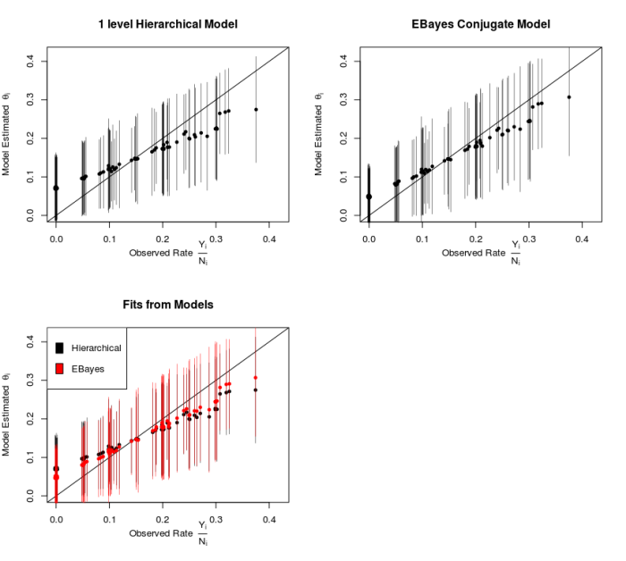
The three panels of the figure show the estimated values of Θ vs the raw observed values. Both models show that the estimated parameters are pulled, shrunk, towards the population means (driven by the prior and sharing of information), and experiments with fewer observations/data are shrunk more.

We may perform model checking by using posterior predictive distributions. New data for a particular experiment i may be simulated, by taking a sample from the posterior distribution of  ; while future experimental data may be generated by drawing a value for Alpha and Beta from the joint posterior sample, and then drawing a new theta and then draw a new data point.

Two Level Model:

This time we use a two level model, from Chapter 9 of [1]. The beta distribution is parameterized using two different, still intuitive parameters:

• Omega ω: which is the location parameter or the proportion of successes.
• Kappa κ: which is the concentration parameter (or opposite of scale) – where large values of kappa will mean that the data is concentrated close to omega (i.e. any values of theta generated from the beta distribution will have a smaller variance). Higher the kappa, the higher our certainty in dependence of theta on omega.

The data I show here is from [1], and consists of baseball players hits and number of times they batted, plus a higher level grouping for each players position. The model has a likelihood and two additional levels: Likelihood, Player Positions, and top level distribution (signifying professional baseball players in general). Figure 9.13 in [2] has a nice diagram to show the structure of the model.

I first model the data using Stan in a two level model, and then use a one level model from the previous section, to model the data at the Position level. The tracking of variables can get a bit tedious in these models, so attention needs to be paid when mapping parameters to the data – with debugging and testing of the code may be required.

I try and reproduce one panel of the Figure 9.14 from [1], showing the group level estimated parameters for players playing at positions Pitcher and Catcher.

If we look at the lower level parameters i.e. individual player estimates from the same group, we can see the affect of shrinkage. The panel on the left shows two pitchers, with same number of trials (about 18/61 and 4/61), but their estimates are shrunk towards the higher level mode (Pitchers), so the difference between their performances spans zero and goes into negative. The panel on the right are two centre fielders (194/593 and 21/120), due to larger data sets the shrinkage is less in this case.

Next we merge the lower level data, i.e. merge the individual player data from each position, and fit a one level model. Here I also try to use an optimisation based approach for parameter estimation, and it appears to converge (however it did not converge in the Rat data set due to the number of parameters that needed tracking) – see [4] for more examples and R code.

### define log posterior
mylogpost = function(theta, data){
  ## parameters to track/estimate
  iTheta = logit.inv(theta[grep('theta', names(theta))])
  iAlDivBe = logit.inv(theta[grep('logitAlDivBe', names(theta))])
  iAlPlusBe = exp(theta[grep('logAlPlusBe', names(theta))])
  
  ## data, binomial
  iSuc = data$success # resp
  iTotal = data$trials
  groupIndex = data$groupIndex # mapping variable
  iTheta = iTheta[groupIndex]
  
  ### we solve two equations together to get the values for alpha and beta
  # log(alpha/beta) = iLogAlDivBe
  # log(alpha+beta) = iLogAlPlusBe
  # solve them together
  A = iAlDivBe
  B = iAlPlusBe
  iAlpha = B/(1+1/A)
  iBeta = B - iAlpha
  
  # checks on parameters
  if (iAlpha < 0 | iBeta < 0) return(-Inf)
  # write the priors and likelihood
  lp = sum(dbeta(iTheta, iAlpha, iBeta, log=T)) + dbeta(A, 0.5, 0.5, log=T) + dgamma(B, 0.5, 1e-4, log=T)
  lik = sum(dbinom(iSuc, iTotal, iTheta, log=T))
  val = lik + lp
  return(val)
}

## set data and starting values
lData = list(success=dfData.2$Hits, trials=dfData.2$AtBats, groupIndex=as.numeric(dfData.2$PriPos))
## set starting values
s1 = lData$success / lData$trials
names(s1) = rep('theta', times=length(s1))
l = getalphabeta(mean(s1), var(s1))

## logit(alpha/(alpha+beta)) = log(alpha/beta)
s2 = c(logit(l['alpha']/sum(l)), log(sum(l)))
names(s2) = c('logitAlDivBe', 'logAlPlusBe')
start = c(logit(s1), s2)

## test function
mylogpost(start, lData)

fit.2 = mylaplace(mylogpost, start, lData)

> fit.2$converge
[1] TRUE

## lets take a sample from this
## parameters for the multivariate t density
tpar = list(m=fit.2$mode, var=fit.2$var*2, df=4)
## get a sample directly and using sir (sampling importance resampling with a t proposal density)
s = sir(mylogpost, tpar, 5000, lData)
mPositions.opt = logit.inv(s[,1:9])
colnames(mPositions.opt) = levels(dfData.2$PriPos)

 

The figure below shows the position specific estimates (apart from Pitchers) for these 4 ways of estimating the parameters.

 The top left panel models the data at 2 levels, and captures the variation among players within the same sub-group of positions – and shows more shrinkage towards a population mean with slightly larger posterior 95% intervals. The other 3 models are adding the data from each player together, hence effectively removing the uncertainty among players in each sub-group of positions. Furthermore, adding the data for each position increases the amount of data, and hence there doesn’t appear to be any shrinkage.

Why not use a Binomial Regression Model

If the aim of the analysis is to look at binomial data, and perhaps perform a hypothesis test for differences between group – it may be straightforward to use a logistic regression model with Random Effects. Modelling the problem like this is good for conceptual understanding and if you loathe yourself :P. However in certain cases the proportions may be more meaningful, e.g. when estimating the methylation proportions at certain positions in the genome using Bisulphite Sequencing data. I have been working on a Bisulphite Sequencing project recently, which required exploring these models in more detail (more to come on BS Sequencing Quality Checks).