Binary problems, where the outcome can be either True or False are very common in data analysis, from an inference or classification point of view. A previous post on binomial modelling deals with a similar problem, but this time we frame the problem from a regression or generalized linear model (GLM) view point. Previously we dealt with some binomial problems but reported the results in terms of proportions. These proportions are sometimes more intuitive and it may be useful to model the data that way, in certain cases. However as we start adding more predictor variables, which also includes continuous variables, then it may be simpler to use a GLM based approach.
Most of the material that we cover here can be found in more detail in:
[1] Kruschke, J. K. (2014). Doing Bayesian data analysis: A tutorial with R, JAGS, and Stan, second edition. Doing Bayesian Data Analysis: A Tutorial with R, JAGS, and Stan, Second Edition. http://doi.org/10.1016/B978-0-12-405888-0.09999-2
[2] Gelman, A., Carlin, J. B., Stern, H. S., & Rubin, D. B. (2013). Bayesian Data Analysis, Third Edition (Texts in Statistical Science). Book.
[3] Jaynes, E. T. (2003). Probability theory the logic of science. Cambridge University Press (2003)
[4] lme4: Mixed-effects modelling with R. Douglas M. Bates (2010). link
My attempt at humour has named the article Logistic Aggression, instead of Logistic Regression. The aggression part here is to understand what do the regression coefficients mean (to develop an intuitive feel for it). We will attempt to calculate it by hand, which can lead to aggression. In certain cases (see [2] for some examples) where the class proportions at not close to 0 or 1, then we may try and model the data using a simple linear regression approach.
We use the Contraception data set from the mlmRev package in R which is used as an example in Chapter 6 of [4] – some of the figures and analysis represents the workflow and reasoning from [4].
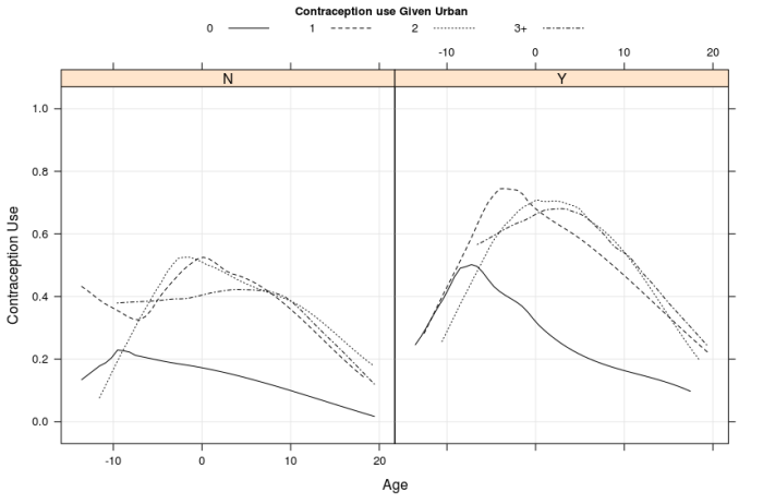
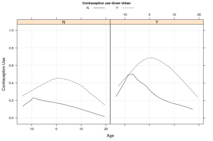 Figure 1: Has two panels top and bottom. Both panels show the contraception use on y axis with respect to age on x axis. The figures suggest that, contraception use and age have a quadratic trend, middle age range users are more likely to use contraception, it is more prevalent in urban areas, users with zero children are less likely to use contraception. The variation among users with more than zero children is small. The bottom panel merges the groups with 1, 2 or 3+ children into one group.
We start the data modelling in steps, first using an odds ratio based approach and then a logistic regression. This should build up the understanding of the meaning of the coefficients. See the chapter on sampling theory and hypothesis testing in [3] for more details on this and some more details are in a previous post.
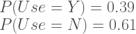
If we do not have any grouping information and using the principle of indifference, we can assign probabilities to contraception Use Y (yes) or Use N (no).
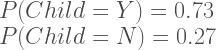
Same can be done for the grouping variable e.g. Children Y or N.
If we look at the conditional distributions of these two variables, also called a contingency table:
| Child=N | Child=Y | |
|---|---|---|
| Use=N | 0.21 | 0.40 |
| Use=Y | 0.07 | 0.32 |
We can see in the table cells, joint probabilities – e.g. Cell 1,1 = 
We have all this information available from our calculations earlier, so plugging them in the Equations 2 and 3 we get:
Snippet 1:
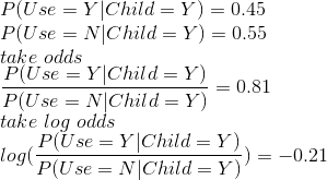
This tells us: the probability of using contraception given a person has a child is 0.45 and probability of not using contraception given the person has a child is 0.55. The odds, given a person has children, of using contraception are less than 1; and log odds are negative which suggests the probability is less than 0.5 (i.e. it is 0.45 in this case).
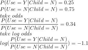
Lets try the second combination, i.e. when we condition on the fact that Child = N. Using the same method as shown in equations 2 and 3:
Snippet 2:
The log odds is basically the same as a logit function, where the domain of the function is from 0 to 1. We are calculating the log odds or logit of the probability that Use=Y given Child=Y in snippet 1 and probability of Use=Y given Child=N in snippet 2. In order to get the original probability back, we use the inverse of the logit function. E.g. we perform a similar calculation as in the snippet 2, but using the logit and inverse logit formulation:

Now on to the easy part, repeating this same analysis in a logistic regression formulation.
> fit.0 = glm(use ~ children, data=Contraception, family = binomial(link='logit'))
> summary(fit.0)

Call:
glm(formula = use ~ children, family = binomial(link = "logit"),
    data = Contraception)

Deviance Residuals:
    Min       1Q   Median       3Q      Max
-1.0866  -1.0866  -0.7602   1.2710   1.6628

Coefficients:
            Estimate Std. Error z value Pr(>|z|)
(Intercept)  -1.0936     0.1002 -10.915  < 2e-16 ***
childrenY     0.8762     0.1137   7.708 1.27e-14 ***
---
Signif. codes:  0 ‘***’ 0.001 ‘**’ 0.01 ‘*’ 0.05 ‘.’ 0.1 ‘ ’ 1

(Dispersion parameter for binomial family taken to be 1)

    Null deviance: 2590.9  on 1933  degrees of freedom
Residual deviance: 2527.0  on 1932  degrees of freedom
AIC: 2531

Number of Fisher Scoring iterations: 4

> ## intercept = log odds of contraception=Y given children=N
> ## convert to probability using logit inverse
> plogis(-1.09) ## compare with snippet 2
[1] 0.2516183
>
> ## log odds of contraception=Y given children=Y (we have switched conditional class)
> ## add intercept and coefficient for children=Y
> round(sum(coef(fit.0)), 2) ## compare with snippet 1
[1] -0.22
> plogis(sum(coef(fit.0)))
[1] 0.4458689
Now this was much simpler, and depending on the nature of the problem and easy of interpretation of results, one would use a regression approach or other approaches to model such problems (one example in previous blog on binomial models).
Model Building and Parameter Estimation:
Some of the steps we perform here, i.e. parameter estimation, model building can be seen in previous blogs (e.g. parameter estimation, model checking). In this post, we won’t touch upon the hierarchical or random effects models – and model everything at the population level. We build the model adding the covariates (following the reasoning in Figure 1 and Chapter 6 of [4]) using the glm function in R, and then using a log posterior function.
fit.1 = glm(use ~ age + I(age^2) + urban + children, data=Contraception, family = binomial(link='logit'))
summary(fit.1)

## lets write a custom glm using a bayesian approach
## write the log posterior function
mylogpost = function(theta, data){
  ## parameters to track/estimate
  betas = theta # vector of betas i.e. regression coefficients for population
  ## data
  resp = data$resp # resp
  mModMatrix = data$mModMatrix

  # calculate fitted value
  iFitted = mModMatrix %*% betas
  # using logit link so use inverse logit
  iFitted = logit.inv(iFitted)
  # write the priors and likelihood
  lp = dnorm(betas[1], 0, 10, log=T) + sum(dnorm(betas[-1], 0, 10, log=T))
  lik = sum(dbinom(resp, 1, iFitted, log=T))
  val = lik + lp
  return(val)
}

mylogpost(start, lData)

fit.2 = laplace(mylogpost, start, lData)

## compare the 2 methods
> data.frame(coef(fit.1), fit.2$mode)
             coef.fit.1.  fit.2.mode
(Intercept) -0.942935490 -0.94214748
age          0.004967476  0.00498954
I(age^2)    -0.004327508 -0.00433278
urbanY       0.766361560  0.76664774
childrenY    0.806217238  0.80593701
We can see that the two methods produce similar results. The second method allows you to customise the regression by adding appropriate priors. We take random samples from this distribution by using the Sampling Importance Resampling approach, using a t proposal density.
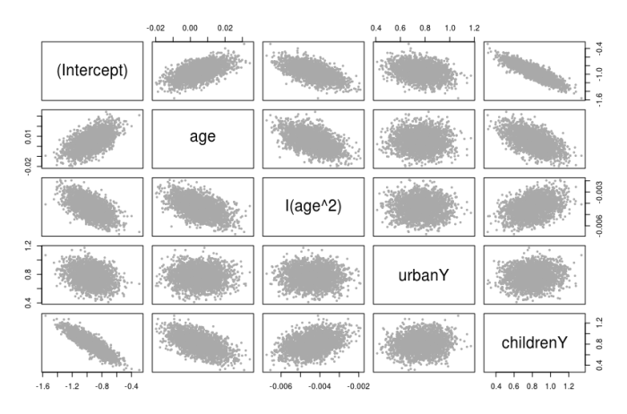
Figure 2: Pairs plot of SIR samples for the parameters in the model.
We can use these pairs plots to perhaps look for correlations between parameters, this also guides us in the process of model building. For example, looking at Figures 1 and 2, there is a relationship between age and children (Y and N) variables: the intercepts, slopes and correlation between these variables suggest an interaction term in the model between age and children (we won’t follow this here for this blog, but these types of plots can guide in the model building process).
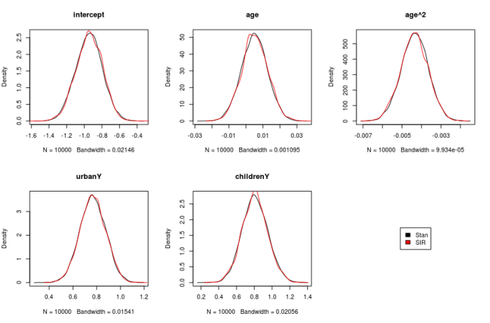
We also repeat this modelling process using Stan, and show the densities obtained using MCMC in Stan and SIR method.
Model Checks:
A more detailed analysis of model checking parameters can be seen on the two previous posts on model checks (1 and 2). Here we are just calculating some predictive scores that include AIC, DIC and WAIC. We calculate it either using the parameters from the MCMC or SIR samples, or directly using the sample of Fitted values from the linear predictor (obtained from Stan directly). Prediction error (misclassification error rate can also be used as a criteria for model checks and may be simpler and more straightforward in certain cases).
## first write the log predictive density function
lpd = function(theta, data){
  betas = theta # vector of betas i.e. regression coefficients for population
  ## data
  resp = data$resp # resp
  mModMatrix = data$mModMatrix
  # calculate fitted value
  iFitted = mModMatrix %*% betas
  # using logit link so use inverse logit
  iFitted = logit.inv(iFitted)
  ## likelihood function with posterior theta
  return(sum(dbinom(resp, 1, iFitted, log=T)))
}

## log pointwise predictive density
lppd = function(theta, data){
  betas = t(theta) # matrix of betas i.e. regression coefficients for population
  ## data
  resp = data$resp # resp
  mModMatrix = matrix(data$mModMatrix, nrow = 1, byrow = T)
  # calculate fitted value
  iFitted = as.vector(mModMatrix %*% betas)
  # using logit link so use inverse logit
  iFitted = logit.inv(iFitted)
  ## likelihood function with posterior theta
  return(mean(dbinom(resp, 1, iFitted, log=F)))
}
The code snippets below show calculations of some of these scores
### distribution for log predictive density
s2 = extract(fit.stan)$betas
fitted = extract(fit.stan)$mu

i = sample(1:5000, size = 1000, replace = F)
## get a distribution of observed log predictive density
s = s2[i,]
lpdSample = sapply(1:1000, function(x) lpd(s[x,], lData))
max(lpdSample) - mean(lpdSample)
[1] 2.403729
## 5/2 = 2.5
# The mean of the posterior distribution of the log predictive density and the difference
# between the mean and the maximum is close to the value of 5/2 that would
# be predicted from asymptotic theory, given that 5 parameters are being estimated. [Gelman 2013]
## calculate this directly
m = fitted[i,]
l = sapply(1:1000, function(x) sum(dbinom(lData$resp, 1, m[x,], log=T)))

max(l) - mean(l)
2.403729

##### another predictive check (AIC)
# AIC
iAIC = (lpd(post, lData) - 5) * -2
iAIC
[1] 2427.873
AIC(fit.1)
[1] 2427.864
Please see the code at github repository for more tests, R and Stan code. In the next blog, we will extend this model to add a Random effects level. There are some special cases where e.g. we have outliers in the data, then a mixture model approach might be appropriate to make the model more robust (I will add a post to robust binomial models sometime later). In certain data sets. if the class separation is very strong then the optimiser may not converge and give warnings that iteration limit has been reached. In that case other models should be explored or perhaps adding more prior information to the coefficients may help. I am giving vague answers here, as this is a problem I will write a blog about sometime. Furthermore, another issue will crop up, when the class proportions are not balanced – e.g. in studying rare events, most of the results will belong to one class. The coefficients in this case may be very unstable, and should be interpreted with care. I would perhaps use a bootstrap based approach, each time selecting equal class proportions for model fitting and then check the coefficients – again this is a vague answer for the time being.
