In a high-throughput experiment one performs measurements on thousands of variables (e.g. genes or proteins) across two or more experimental conditions. In bioinformatics, we come across such data generated using technologies like Microarrays, Next generation sequencing, Mass spec etc. Data from these technologies have their own pre-processing, normalising and quality checks (see here and here for some checks), and eventually we tend to get a data matrix. This matrix can be viewed in either subject or variable space (see here for more on this). The subjects are the number of samples and the variables are the number of genes (or proteins etc – we will just call them genes for convenience) that are measured.
Some of the material covered here will refer to previous posts (that contain original references to literature) and I will add some references here.
[1] Bishop, C. M. (2006). Pattern Recognition And Machine Learning. Springer. http://doi.org/10.1117/1.2819119
[2] Gelman, A., Carlin, J. B., Stern, H. S., & Rubin, D. B. (2013). Bayesian Data Analysis, Third Edition (Texts in Statistical Science). Book.
The analysis can be handled in different ways, depending on the aim of the study, two common ways are:
- In a classification or prediction scenario, where we wish to find a ‘biomarker’ to predict class A from perhaps a 2 class problem (consisting of classes A and B). In this context, the response variable (or output or target variable) is a binary variable with two levels A and B and is of length N (N being the number of samples). The number of predictors or input variables are the number of genes measured, designated as M. In this situation M is much larger than N, which makes it a high dimensional problem. Here you have to deal with various issues, including overfitting and curse of dimensionality [1]. In these types of problems we tend to go down the route of dimension reduction, regularisation and numerous other pattern recognition approaches [1].
- The second scenario is inference and statistical hypothesis testing, where the aim is to check if the average expression level of a gene is statistically different between groups A and B. In this case the response variable is a gene with N measurements and the predictor is a 2 class variable (M=2). This is not a high dimension problem as the number N is larger than M (one may still face issues of overfitting).
In this post, we deal with the second scenario and there is a lot of literature on this, e.g. there are many statistical packages available to model this problem (like Limma, DESeq2, EdgeR etc). Generally this problem is dealt with by fitting M (M = number of genes measured) regression models, where expression level of one gene is the response variable of length N and the main grouping variable (or treatment) is the first covariate and then some control covariates may be added to the model. Usually one fits somewhere around 10 to 20 thousand models (typical number of genes measured), and then calculate P-Values for the coefficients or differences in coefficients for the treatment (with multiple testing corrections).
Ideally these genes should be modelled together, in a hierarchical model with the variance components of the regression coefficients shared, but this can be computationally intensive. Therefore, some of the statistical packages will use an Empirical Bayes approach to calculate the hierarchical variance hyperparameters for a prior distribution on the variance of the coefficients. This allows sharing of information between the genes through the prior variance for the coefficients in all the models. Sometimes this approach may not be necessary if N is fairly large, as the data dominates the prior, and the practical differences between using an Empirical Bayes approach or not are minimal.
If one had time, computational resources and could be bothered then one can also use a hierarchical model to perform the same analysis in one model where the hyperparameters are estimated (instead of fixed) using a hyperprior distribution and fixed hyper-hyperprior parameters (adding another hyper tends to blow my mind). Imagine a matrix of size N X M. If we stack this matrix into one long vector where the length of the vector is N X M – while the data for each gene can be identified by a mapping variable (factor with M levels) and similarly the data for each treatment can be identified by a second variable (factor with 2 levels in our case A and B). We can identify each unique coefficient by an interaction between the Gene and Treatment factors.
Let us show this by an example to make it more clear. We use part of a microarray data set, consisting of repeated measurements in patients suffering from Tuberculosis and undergoing treatment. The measurements are taken at time points 0, 2 and 12 months. Details about this dataset can be found here. I have provided a sample of this data and the analysis scripts on the github page here.
> m = lData$data
> dim(m)
# matrix with 19329 Genes and 21 Samples
[1] 19329    21

## stack this into one vector
dfData = data.frame(t(m))
dfData = stack(dfData)
dfData$fBatch = lData$cov1
dfData$fAdjust = lData$cov2
## interaction between treatments and genes
dfData$Coef = factor(dfData$fBatch:dfData$ind)
## interaction between control factor and genes
dfData$Coef.adj = factor(dfData$fAdjust:dfData$ind)

> str(dfData)
'data.frame':   405909 obs. of  6 variables:
 $ values  : num  14.6 14.6 14.5 14.2 14.4 ...
 $ ind     : Factor w/ 19329 levels "EEF1A1","GAPDH",..: 1 1 1 1 1 1 1 2 2 2 ...
 $ fBatch  : Factor w/ 3 levels "12","2","0": 1 1 1 1 1 1 1 1 1 1 ...
 $ fAdjust : Factor w/ 7 levels "tr002","tr007",..: 1 2 3 4 5 6 7 1 2 3 ...
 $ Coef    : Factor w/ 57987 levels "12:EEF1A1","12:GAPDH",..: 1 1 1 1 1 1 1 2 2 2 ...
 $ Coef.adj: Factor w/ 135303 levels "tr002:EEF1A1",..: 1 19330 38659 57988 77317 96646 115975 2 19331 38660 ...
We first fit about 19,000 models using Limma, and extract the difference (log Fold Change, abbreviated LFC) between the coefficients for measurement at month 12 and month 2. We then repeat this same process but in one hierarchical model using lme4 library.
library(limma)

design = model.matrix(~ lData$cov1 + lData$cov2)
fit = lmFit(lData$data, design)
fit = eBayes(fit)
## extract the coefficients
dfLimmma.2 = topTable(fit, coef=2, adjust='BH', number = Inf)

########### fit one hierarchical model using lmer
library(lme4)
fit.lme1 = lmer(values ~ 1 + (1 | Coef) + (1 | Coef.adj), data=dfData, REML=F)
summary(fit.lme1)

Random effects:
 Groups   Name        Variance Std.Dev.
 Coef.adj (Intercept) 0.02607  0.1615
 Coef     (Intercept) 3.40543  1.8454
 Residual             0.08203  0.2864
Number of obs: 405909, groups:  Coef.adj, 135303; Coef, 57987

Fixed effects:
            Estimate Std. Error t value
(Intercept) 5.401893   0.007689   702.5
We fit another model using Stan as shown below, and use the initial values calculated using lme4 (NOTE: Fitting the model using Stan can take a few hours on my desktop, so debug and test it on a subset of the data, then perhaps leave it running overnight on a full dataset).
## fit model with stan
library(rstan)
rstan_options(auto_write = TRUE)
options(mc.cores = parallel::detectCores())

stanDso = rstan::stan_model(file='normResponse2RandomEffectsNoFixed.stan')

## calculate hyperparameters for variance of coefficients
l = gammaShRaFromModeSD(sd(dfData$values), 2*sd(dfData$values))
# ## set initial values from lme4 object
ran = ranef(fit.lme1)
r1 = ran$Coef
r2 = ran$Coef.adj
initf = function(chain_id = 1) {
  list(sigmaRan1 = 2, sigmaRan2=2, sigmaPop=1, rGroupsJitter1=r1, rGroupsJitter2=r2)
}

### try a t model without mixture
lStanData = list(Ntotal=nrow(dfData), Nclusters1=nlevels(dfData$Coef),
                 Nclusters2=nlevels(dfData$Coef.adj),
                 NgroupMap1=as.numeric(dfData$Coef),
                 NgroupMap2=as.numeric(dfData$Coef.adj),
                 Ncol=1,
                 y=dfData$values,
                 gammaShape=l$shape, gammaRate=l$rate,
                 intercept = mean(dfData$values), intercept_sd= sd(dfData$values)*3)

fit.stan = sampling(stanDso, data=lStanData, iter=500, chains=4,
                    pars=c('sigmaRan1', 'sigmaRan2', 'betas',
                           'sigmaPop',
                           'rGroupsJitter1', 'rGroupsJitter2'),
                    cores=4, init=initf)
The coefficients we are interested in are in the components of the vector rGroupsJitter1, (or equivalently in the Random Effects coefficients of the lme object) which will be equal to the number of levels of the factor dfData$Coef. We can extract these coefficients from the fit.stan object and use the MCMC sample for each coefficient to calculate a standard deviation and a P-Value (the scripts are in the github repository).
The next few figures below show a comparison between the results from the two models i.e. the Limma based models and Stan based model (the coefficients extracted from the lme4 object should also be comparable).

Figure 1: 2 Panels showing the volcano plots for the differences between expression levels at month 2 and 12 (12 is the baseline). The Red coloured dots represent the genes that show up as statistically significant at a false discovery rate (FDR) of 10%.
Figure 1 shows two main differences between the analysis done by Limma and Stan, due to the variance hyperparameter being estimated and modelling the data together : 1) The shrinkage of coefficients is more apparent in Stan model; 2) The most significant genes (or coefficients) in the analysis have very small standard errors and stand out more in the Stan model than the Limma model. Interestingly the top candidates, from our previous work on TB biomarkers, overlap with the top genes identified by Stan.
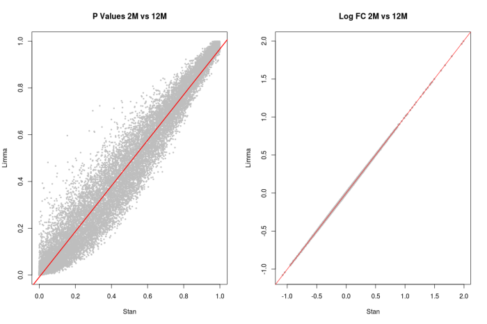
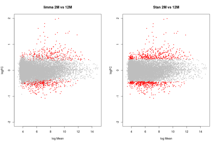 Figure 2: The 4 panels show the comparisons between the Stan and Limma models, and they appear to be in agreement.
We can also perform a quick sanity check with a pathway analysis (e.g. Reactome database) using a list of top 100 genes (sorted on P-Values in ascending order) to check for the similarity of results as shown in Table 1:
Table 1: Top 12 pathways showing significant over-representation of the top 100 Genes selected from Limma and Stan analysis.
| Stan | Limma |
|---|---|
| Cytokine Signaling in Immune system | Cytokine Signaling in Immune system |
| Interferon Signaling | Interferon Signaling |
| Immune System | Immune System |
| Interferon alpha/beta signaling | Interferon alpha/beta signaling |
| Interleukin-4 and 13 signaling | Interferon gamma signaling |
| CLEC7A/inflammasome pathway | CLEC7A/inflammasome pathway |
| Signaling by Interleukins | Antiviral mechanism by IFN-stimulated genes |
| Interleukin-10 signaling | ISG15 antiviral mechanism |
| Interferon gamma signaling | Innate Immune System |
| RUNX1 regulates transcription of genes involved in BCR signaling | RUNX1 regulates transcription of genes involved in BCR signaling |
| Fibronectin matrix formation | Fibronectin matrix formation |
| TNFs bind their physiological receptors | Signaling by Interleukins |
The drawback of using the Stan based model is the complexity and computation time; while the advantages in the current case appear to be clearly showing a separation in the most significant genes while this separation is not as strong in the Limma based model. Furthermore, one model makes the posterior predictive model checks and model comparisons more straight-forward. Understanding this model is also a good intellectual exercise and can be applied in other areas and types of data. This is particularly useful when the response variable may require a distribution other than normal e.g. a heavy tailed distribution to accommodate outliers.
Continuing along this line, we try a heavy tailed distribution, i.e. a t distribution where we set the normality parameter (or degrees of freedom very low – actually we let Stan estimate it, but you can fix it to something like 4 as well) [2]. This model is very slow to converge but one can see differences in the results.

Figure 3: A volcano plot similar to Figure 1, but this time using a T distribution for the likelihood or data distribution. There is less shrinkage in the coefficients and we can still see the top genes that are known biomarkers for tuberculosis diagnosis.
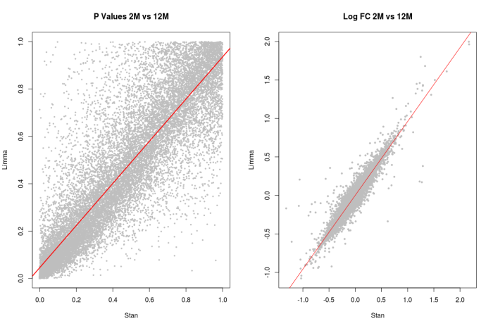
Figure 4: Similar comparison to Figure 2, and we can see more differences between the Limma and Stan model with a heavy tailed distribution. Generally the results overlap, but differences will be present in Genes with outlier measurements.
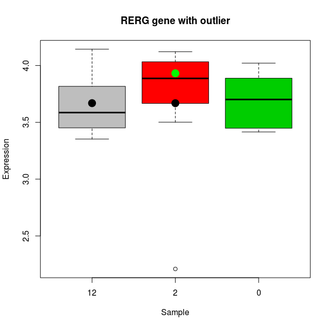
Figure 5: One of the genes (RERG) that shows differences in fold changes calculated from Limma and Stan. The x axis shows the three groups (12, 2 and 0 months since start of treatment), the y axis shows the expression levels. The black dot on the 12 month box plot show the location of the grand mean or intercept. The black dot on the 2 months sample shows the location of the 2 months group average calculated through Limma; this average is pulled down due to the outlier measurement (see dot at around 2.2) and infact the fold change calculated is negative (-0.0003). The green dot however shows average calculated using Stan (with a heavy tailed distribution), and the outlier sample is not influencing the fold change (which is positive ~ 0.26).
If one expects a lot of outliers in the data, then a heavy tailed distribution would be more appropriate – especially if the fold changes are to be used in some downstream enrichment analysis.
